Tutorial 2: Filtering and Pre-Processing

This notebook shows how to pre-process and filter trajectory dataframes using nomad. The nomad library currently provides functions for coordinate-system projection, and spatial, temporal, and quantity filtering.

import pandas as pd
import numpy as np
import matplotlib.pyplot as plt
from shapely.geometry import Polygon
from datetime import datetime
import matplotlib.patches as patches
from pyproj import Transformer

import nomad.io.base as loader
import nomad.filters as filters
from nomad.filters import to_projection, filter_users
import nomad.city_gen as cg

Load Data

For the following examples, we load test data from nomad.

raw_traj = loader.from_file('../nomad/data/gc_sample.csv', format='csv')
raw_traj.head(10)

	uid	timestamp	tz_offset	longitude	latitude
0	wizardly_joliot	1704120060	-18000	38.321669	-36.667588
1	wizardly_joliot	1704122760	-18000	38.321849	-36.667467
2	wizardly_joliot	1704124380	-18000	38.321752	-36.667464
3	wizardly_joliot	1704137280	-18000	38.321629	-36.667374
4	wizardly_joliot	1704138780	-18000	38.321636	-36.667238
5	wizardly_joliot	1704139740	-18000	38.321654	-36.667281
6	wizardly_joliot	1704140340	-18000	38.321641	-36.667338
7	wizardly_joliot	1704143280	-18000	38.321589	-36.667410
8	wizardly_joliot	1704143400	-18000	38.321687	-36.667524
9	wizardly_joliot	1704143580	-18000	38.321703	-36.667460

Project between coordinate systems

Many geospatial datasets come in spherical coordiantes latitude/longitude (EPSG:4326). However, spatial analyses---like joins of points in polygons, computing buffers, or clustering pings---might benefit from computing euclidean distances. Thus projected planar coordinates (like EPSG:3857) are commonly used. Nomad's to_projection method creates new columns x and y with projected coordinates in any coordinate reference system (CRS) recognized by PyProj.

# Project to EPSG:3857 (Web Mercator)
projected_x, projected_y = to_projection(traj=raw_traj,
                                         input_crs="EPSG:4326",
                                         output_crs="EPSG:3857",
                                         longitude="longitude",
                                         latitude="latitude")

traj = raw_traj.copy()
traj['x'] = projected_x
traj['y'] = projected_y

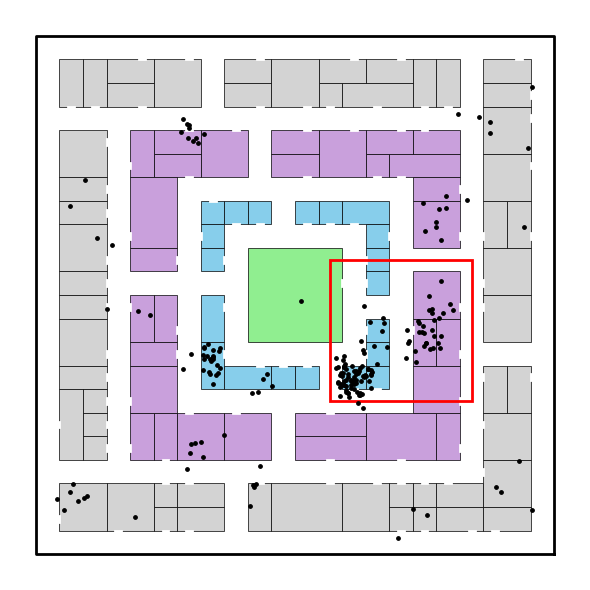
The following code visualizes the trajectory. We transform the coordinates in the sample data back to the Garden City coordinates (in a 22x22 box) so that we can visualize the city buildings alongside the blocks. The red box depicts the area we will filter to.

plot_df = traj[traj['uid'] == "agitated_chebyshev"].copy()
transformer = Transformer.from_crs("EPSG:4326", "EPSG:3857", always_xy=True)
plot_df['x'], plot_df['y'] = transformer.transform(plot_df['longitude'].values, plot_df['latitude'].values)
plot_df['x'] = (plot_df['x'] - 4265699)/15
plot_df['y'] = (plot_df['y'] + 4392976)/15

fig, ax = plt.subplots(figsize=(6, 6))
plt.box(on=False)

# Plotting Pings
ax.scatter(x=plot_df['x'], 
           y=plot_df['y'],
           s=6,
           color='black',
           alpha=1,
           zorder=2)

# Plotting Garden City Map
city = cg.load('garden-city.pkl')
city.plot_city(ax, doors=True, address=False)

polygon_coords = [
    (12.5, 12.5), 
    (12.5, 6.5), 
    (18.5, 6.5), 
    (18.5, 12.5)
]
polygon = Polygon(polygon_coords)

polygon_patch = patches.Polygon(polygon.exterior.coords, closed=True, edgecolor='red', facecolor='none', linewidth=2, label="Polygon")
plt.gca().add_patch(polygon_patch)

ax.set_yticklabels([])
ax.set_xticklabels([])
ax.set_xticks([])
ax.set_yticks([])

plt.tight_layout()
plt.show()

png

Filter to a specified geometry

We often need to filter down the dataset to the most relevant records. This involves filtering along three key dimensions: - Spatial Filtering: Keep only users with pings that fall within a specific geographic region (e.g., Philadelphia). Use the polygon argument. - Temporal Filtering: Restrict data to a time window of interest (e.g., January). Use the start_time and end_time arguments. If - Quantity-Based Filtering: Keep only users with sufficient activity as measured by a minimum number of pings. Use the min_active_days and min_pings_per_day arguments.

If the aforementioned arguments are not specified, the default arguments ensure that the respective filtering is not performed. E.g., polygon defaults to None, and so no spatial filtering is performed.

These filtering functions help clean and prepare your dataset for downstream analysis by focusing only on users who are present, active, and engaged in the geographic area and timeframe you care about.

polygon_coords = [
    (4265886.5, -4392788.5), 
    (4265886.5, -4392878.5), 
    (4265976.5, -4392878.5), 
    (4265976.5, -4392788.5)
]
polygon = Polygon(polygon_coords)

n0 = len(traj)
uq0 = traj['uid'].unique()

filtered_traj = filter_users(traj=traj, 
                             start_time="2024-01-01 00:00:00",
                             end_time="2024-01-31 23:59:00",
                             polygon=polygon,
                             min_active_days=2,
                             min_pings_per_day=10,
                             user_id='uid',
                             x='x',
                             y='y')

n1 = len(filtered_traj)
uq1 = filtered_traj['uid'].unique()
print(f"Number of pings before filtering: {n0}")
print(f"Number of unique users before filtering: {len(uq0)}")
print(f"Number of pings after filtering: {n1}")
print(f"Number of unique users after filtering: {len(uq1)}")

Number of pings before filtering: 26977
Number of unique users before filtering: 100
Number of pings after filtering: 15912
Number of unique users after filtering: 35